Modeling
This section describes how to perform Finite Element Method (FEM) analysis of our PneuNet actuator using the Abaqus software suite. FEM allows us to model the behavior of the actuator and see the effects of changing various parameters such as material stiffness or chamber dimensions, without needing to refabricate and retest the actuator every time a design parameter is changed.
The Abaqus input file created in this tutorial can be downloaded here and the .STEP files of the actuator can be downloaded here.
Overview of model components
- A Fluid-Structure Interaction (FSI) problem treated with a standard/implicit FEM using Abaqus/CAE (SIMULIA, Dassault Systèmes)
- 2 materials:
- Elastosil M4601 silicone rubber: Yeoh strain energy potential defined by the coefficients C10 = 0.11, C20 = 0.02. Density of 1130 Kg/m³, assumed isotropic
- Paper: density of 750 Kg/m³, a Young’s Modulus of 6.5 GPa and a Poisson’s ratio of 0.2
- 2 sections:
- Elastosil (uniform solid), assigned to the main body and 2 bottom layers
- Paper (uniform shell), assigned to inextensible layer
- 2 loads:
- Gravity, with boundary condition as 1 end rigidly fixed (encastre)
- Pressure, acting at all internal faces of the actuator cavity
- Contact interaction between adjacent chamber walls
Overview of FEM steps
- Import parts
- Make surface placeholder for paper layer
- Assign material properties to the parts (create materials, assign materials to sections, assign sections to parts)
- Assemble parts
- Model paper layer as a skin and assign final section
- Create a surface on inner cavity faces
- Apply loads (gravity, and pressure on inner cavity) and set boundary conditions
- Add contact interaction
- Create mesh and run job
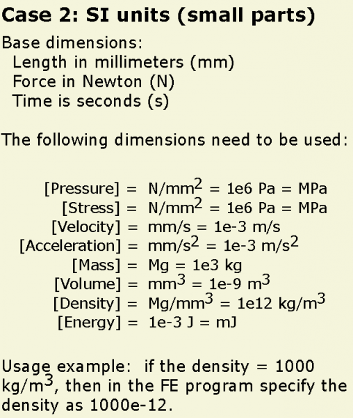
A note on units
Abaqus doesn’t interpret units so it is up to the user to make sure they are consistent. In this tutorial we use the following scheme:
| PneuNets Abaqus CAE input file | 2.73 MB | |
| Modified for Abaqus - PneuNet Molds .STEP Files (.zip) | 40 KB |
Create parts and assign materials
Import parts
[Video: Import parts and make paper surface]
 |
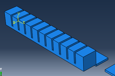
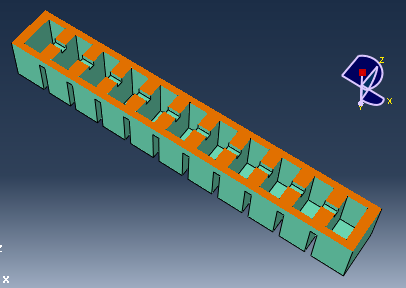
The generic design of these actuators consists of two different materials; the elastomer parts and an elastomer embedded inextensible part (layer of paper) at the bottom of the actuator. This layer causes the actuator to bend as it minimizes axial expansion. |
In order to make the simulation less computationally expensive, the actuator geometry is simplified by omitting certain features – i.e. the bonding ridges/bumps at the bottom the main body.
The .STEP files of the actuator geometry used in this tutorial can be downloaded here. If you would like to modify/customize the geometry, the SolidWorks part files of the simplified actuator can be downloaded here.
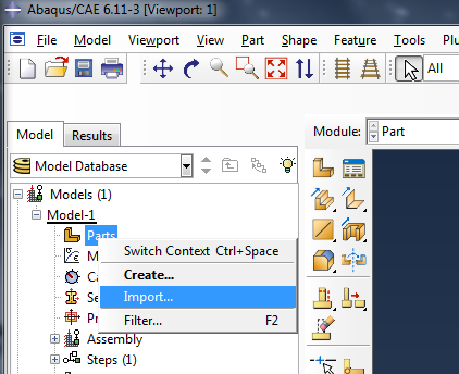 |
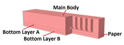
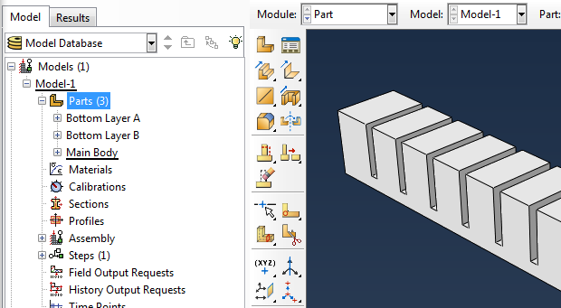
Import your CAD parts (as .STEP files) – here we have 3 parts, the Main Body plus Bottom Layers A & B. To do this, go to the model tree in the left sidebar, right-click on "Parts" and select Import. Browse to the .STEP file. |
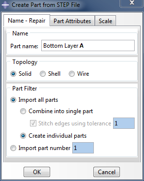 |
Name the part, and make sure to import it as a Solid. |
Repeat with the remaining 2 parts. All the parts should now appear in the model tree.
Create a placeholder for the inextensible layer
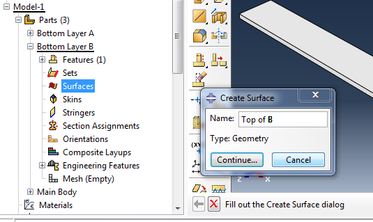
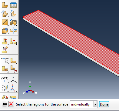
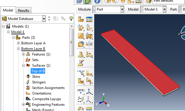
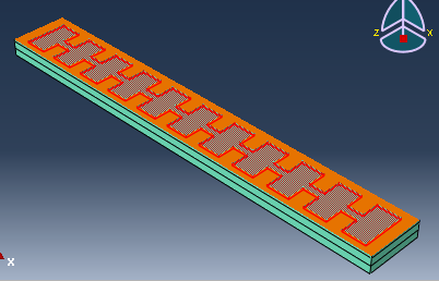
To model the piece of paper, return to the part list in the model tree and expand 'Bottom Layer B.' Double click on Surfaces and select the upper face of the part to create a surface there.
  |
Create material: paper
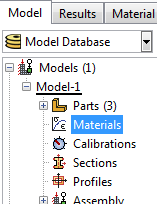 |
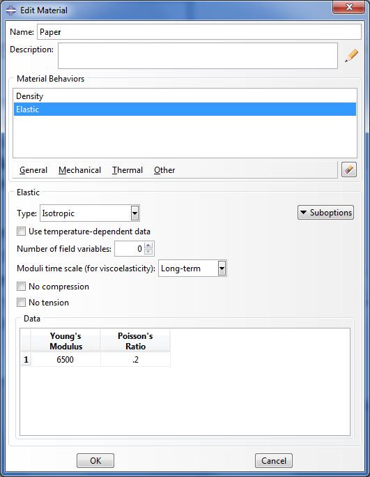
Before assigning material properties, we first create the necessary materials. We need two materials: paper, and the elastomer (Elastosil). In the model tree, double click on Materials to create a new material, and name it ‘Paper.’ |
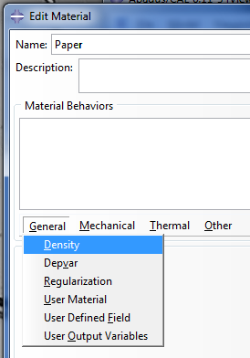
Set the following properties:
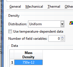
- General > Density:
- Density = 750 Kg/m³ → 750e-12 (Mg/mm³)
- Mechanical > Elasticity> Elastic:
- Young’s Modulus = 6.5 GPa → 6500 (MPa)
- Poisson’s ratio = 0.2
  |
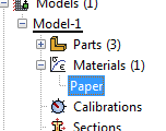
Paper should now appear under Materials in the model tree.
Create material: Elastosil
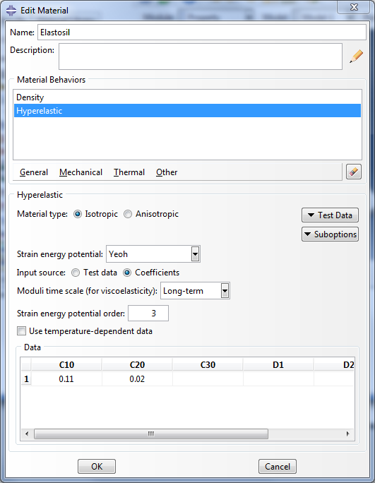
For the Elastosil, set:
- General > Density:
- Density = 1130 Kg/m³ → 1130e-12 (Mg/mm³)
- Mechanical > Elasticity > Hyperelastic:
- Strain energy potential = Yeoh
- Input source = Coefficients
- C10 = 0.11, C20 = 0.02
- Assume isotropic material type
Create sections
[Video: Create and assign sections]
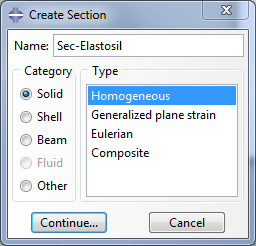
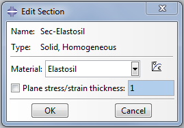
Double click on Sections in the model tree to create a new section. Set it to be a homogeneous solid and assign Elastosil as the material.
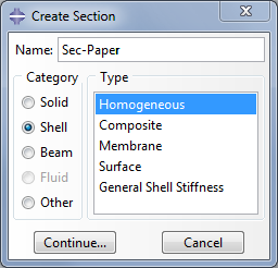
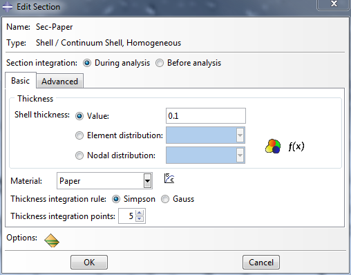
Create another section, a homogeneous shell with paper assigned as the material. Set the shell thickness to 0.1
  |
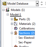
You should now have 2 sections in your model tree.
Assign sections to parts
Go back to the parts you imported and assign a section to each one. To do this, look under each part in the model tree and double click on Section Assignments. Select the entire part geometry, then assign the Elastosil section.
| Modified for Abaqus - PneuNet Molds .STEP Files (.zip) | 40 KB | |
| Modified for Abaqus - PneuNet Molds SolidWorks Files (.zip) | 257 KB |
Assemble and merge
Create assembly
[Video: Assemble with constraints]
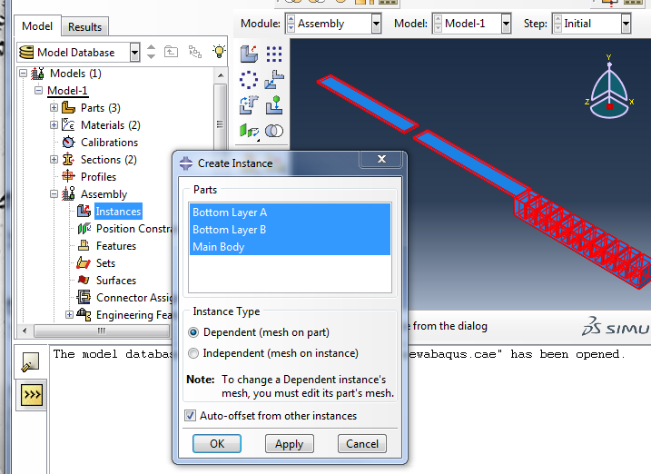
Now we assemble all the individual parts. In the model tree, expand Assembly, double click on Instances and select all 3 parts. Instance Type should be set to "Dependent".
Checking “Auto-offset from other instances” is also helpful as Bottom Layer A & B have identical shapes and positions and overlap each other, making them hard to distinguish. Alternatively, you can manually translate one of the overlapping parts.
Position parts
Now the parts have to be positioned properly relative to each other. To do this 6 total constraints are needed: 3 translational DOF for each of 2 parts, relative to one fixed part.
Use the face-to-face tool to “mate” faces like you would in SolidWorks (hold down the parallel faces button until another menu appears).
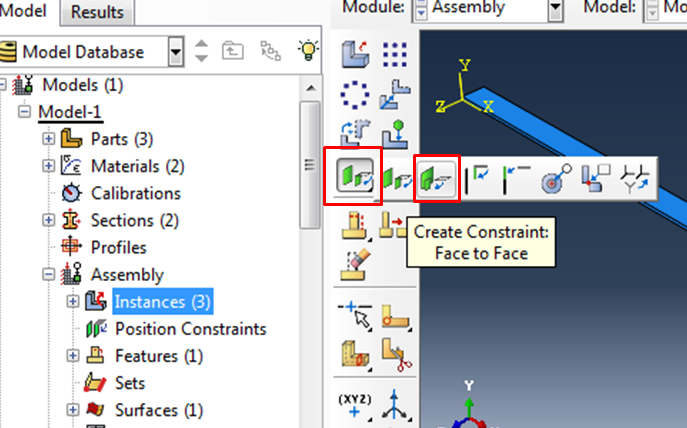
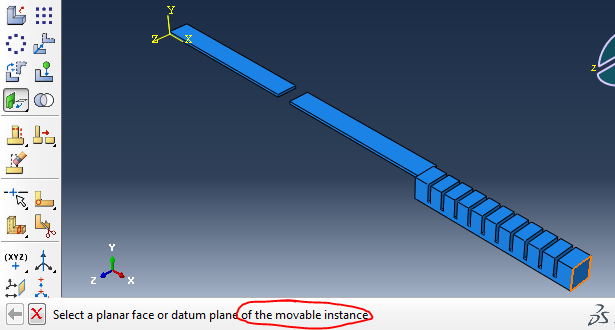
With this tool, you select the two faces you want to mate. the order in which you select faces is important: one of the parts is designated as movable, and the other as fixed. As you add more constraints, you should be consistent about the part you choose to be fixed, otherwise you will create a dependency cycle and get an error.
Here we will treat Bottom Layer A as fixed, and move the other parts relative to it.
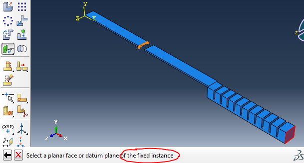
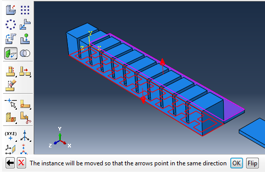
The 2 arrows that appear should be pointing in the same direction (click on “Flip” if they aren’t).
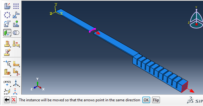
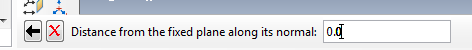
Next, set ‘Distance from the fixed plane along its normal’ to 0 and hit Enter. This completes the constraint and the movable part has changed its position.
When mating the bottom face of the Main Body to the top face of Layer A, the arrows will initially point in opposite directions. Click the Flip button to make them point in the same direction.

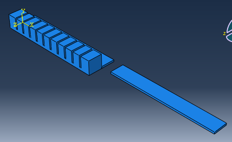
Repeat until all parts are in place.
Merge
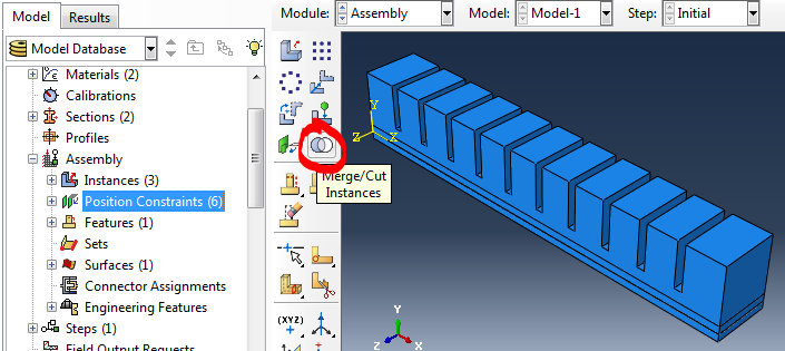
Under the assembly module toolbar, click the Merge/Cut Instances button.
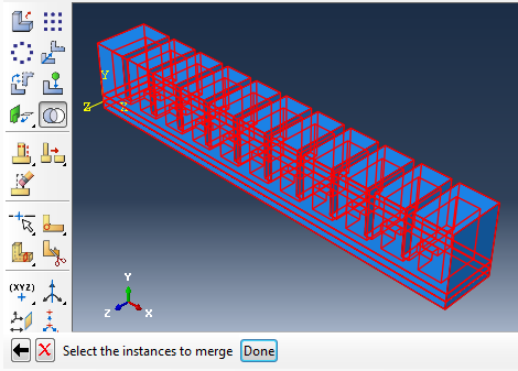 |
Select the entire assembly, and click Done. |
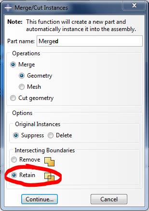 |
In the new window, make sure to use the ‘Retain’ option for intersecting boundaries. A new part, the merged part, will be created in the parts list. |
Create inextensible layer
Select surface to skin
[Video: Create skin and assign paper section]
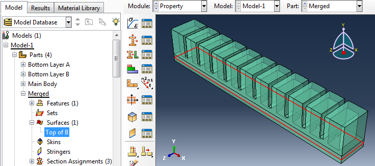
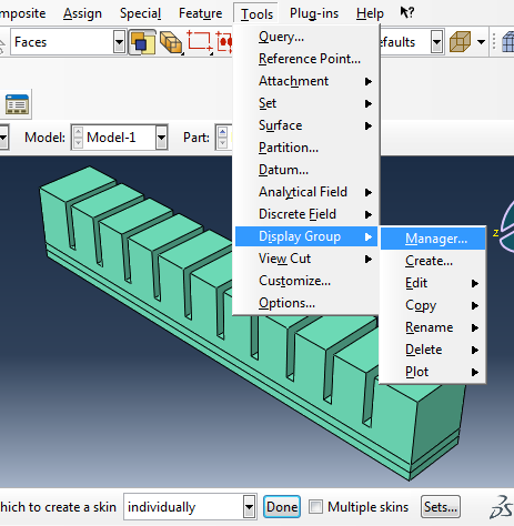
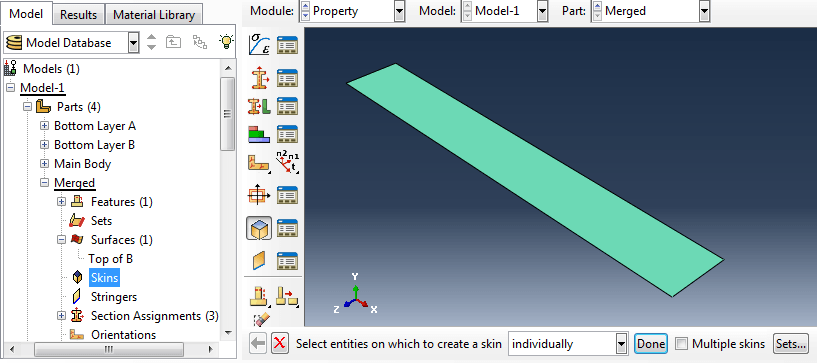
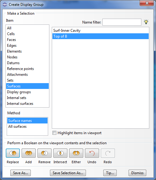
We also need to finish modeling the inextensible paper layer. Go back to the merged part and click to create a Skin. The software will ask you to select the entity on which it will create the skin. We want to select the surface of the ‘Bottom Layer B’ that we created beforehand, but right now it is buried under other parts. To isolate it, you will have to go to: Tools → Display Group → Manager.
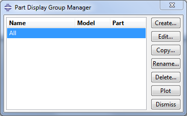
The ‘Part Display Group Manager’ will appear – select Create.
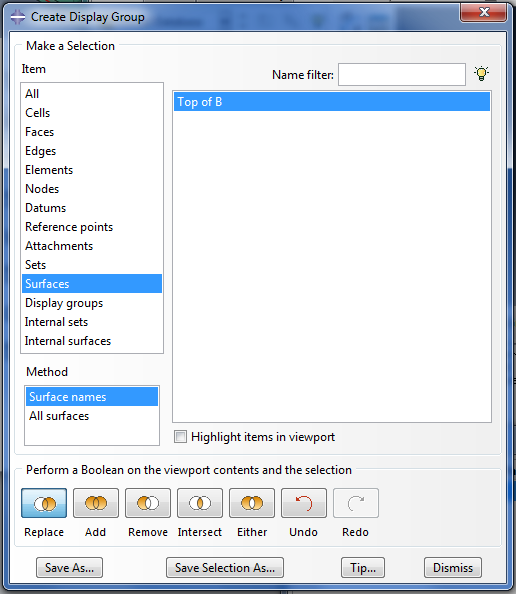
The ‘Create Display Group’ will now come up – select ‘Surfaces’ and click on the paper surface from the list and then ‘Replace’ and ‘Dismiss’.
This will make only this surface visible in the view. Select the top face of the surface to create the skin.
Assign section
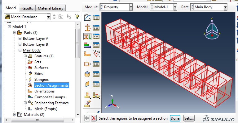
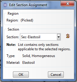
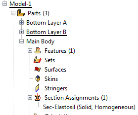
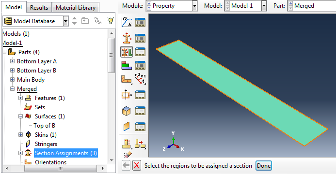
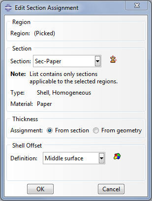
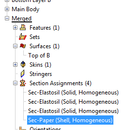
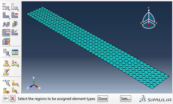
While at the Merged part, click on the ‘Section Assignment’. There you should already have three sections (all Elastosil). To create a new section for the paper double click the ‘Section Assignment’ and then select the region to be assigned a property by clicking again on the top surface. The ‘Edit Section Assignment’ window will appear where you should select the Paper as the Section. Make sure the Type is ‘Shell, Homogeneous’. Click OK. You have successfully created one more section assignment for the paper.
Create loads
Select the inner cavity surface
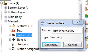 |
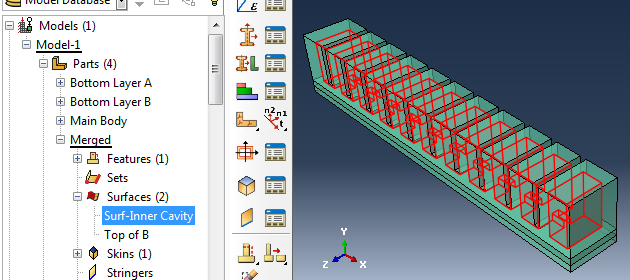
[Video: Select inner cavity surface] Before we start adding loads, we need to define the surface that the pressure load will act upon. This surface is made up of all the faces of the inner cavity of the actuator. To create this surface, expand the Merged part in the model tree and double-click on Surfaces. Name it something like “Surf-Inner Cavity.” |
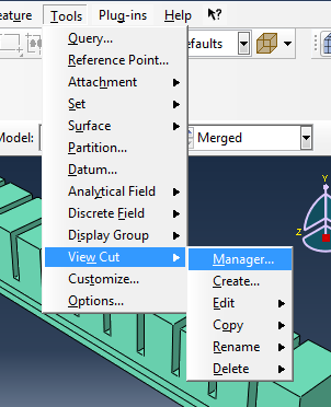
Now we have to select the faces that make up this surface. However, since the cavity is not accessible, use the Cross Section views provided from Tools > View Cut > Manager. Section using the Y-plane to expose it.
|
|
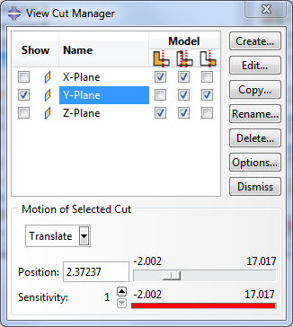
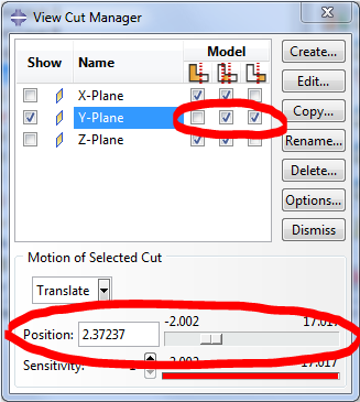
Reposition the cut until both the inner chambers and the central channel are exposed, and flip the cut so that the ceilings of the chambers are visible.
|
|
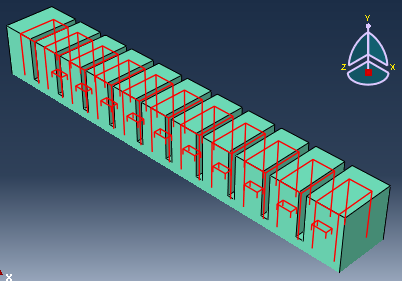 |
Holding down SHIFT, click to select all the available faces of the inner cavity. This includes 4 sidewalls + ceiling for each chamber and 3 faces of each channel. You will have to rotate your view at least twice to be able to select everything. |
 |
Finally, reverse the view cut and select the floor of the inner cavity. This completes the surface. |
Create gravity step
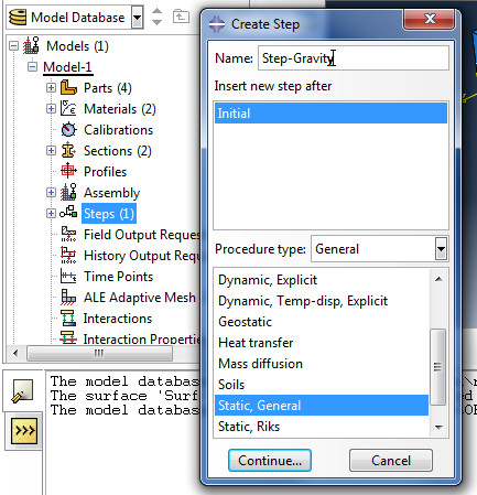 |
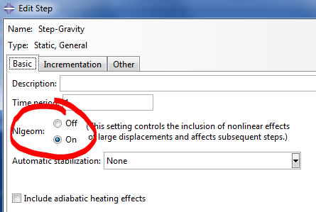
In the model tree, double-click on Steps to create the first step that accounts for the gravity acting on the actuator. Select a ‘Static, General’ procedure type and in the next window turn ON the ‘Nlgeom’ option. |
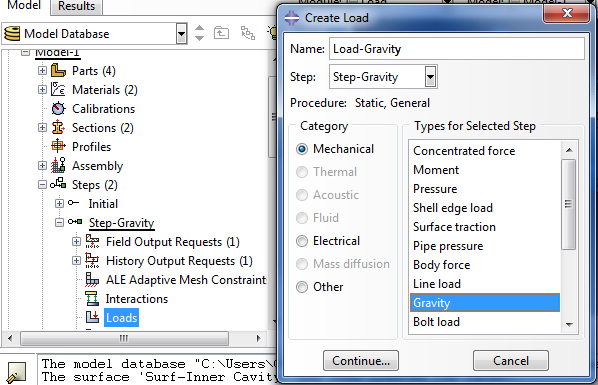
Set gravity load
Under the gravity step, double-click Loads and activate Gravity as the selected type for the step.
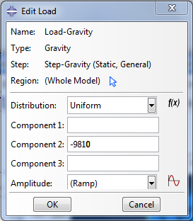 |
Set the gravity value, as -9810 on the Y axis/Component 2. |
Set gravity load boundary conditions
Click on BCs (boundary conditions), and select Symmetry/Antisymmetry/Encastre.
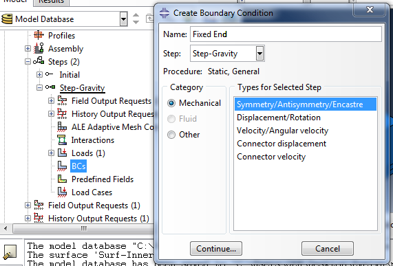
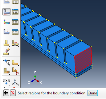
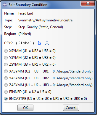
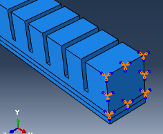
Continue and click on the face of the part that is going to be fixed. Select ‘Encastre’ to fix the surface.
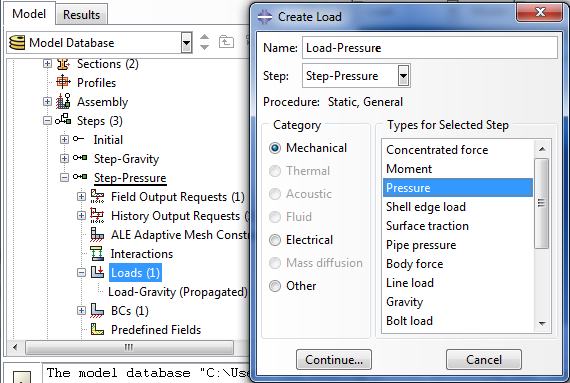
Create pressure step
Create a second step by double-clicking on Step again, making it ‘Static, general’ again.
This step will have all the attributes of the previous step propagated to it and the pressure inside the cavity of the actuator will be enabled here. Within the second step, create a Pressure load.
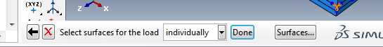
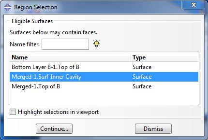
To pick the internal cavity click the ‘Surfaces’ button at the bottom right corner. In the Region Selection window that appears, select the surface "Surf-Inner Cavity" which we created earlier.
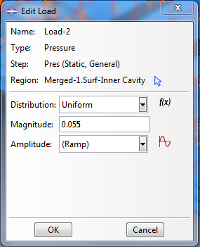
At the next window provide the pressure value to be applied in the cavity. This PneuNet design curls fully with 8 psi, which is approximately 55 kPa. Since our units should be in MPa, we use 0.055 MPa.
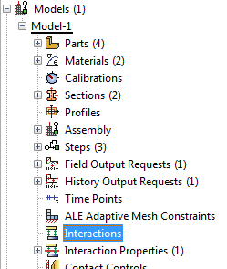
Add contact interaction
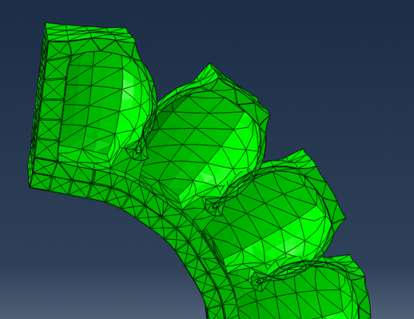
When a PneuNet is sufficiently inflated, the walls of adjacent chambers will come into contact with each other. However, Abaqus explicitly needs to be told to take this physical interaction into account; otherwise, the modeled result will have the walls simply passing through each other, as seen below:
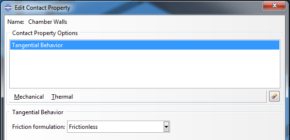
Create interaction property
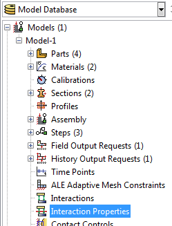
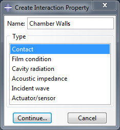
First, we create the type of interaction we want to model. In the model tree, double click on Interaction Properties and create a new property of the type "Contact."
  |
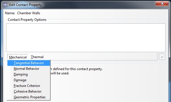
Add Mechanical > Tangential Behavior from the dropdown menu, and make it frictionless.
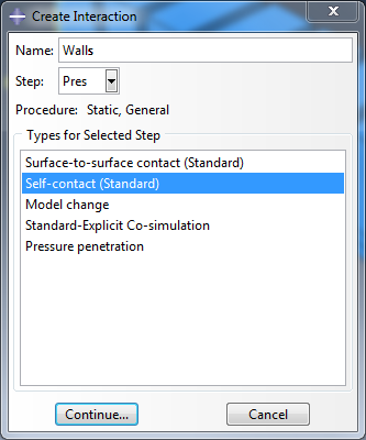
Create interaction
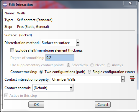
Now we define where/how the above interaction type is going to apply. In the model tree, double-click on Interaction and create a new interaction of type "Self-contact (Standard)." Make sure that this interaction applies during the Pressure step, since that is when the walls begin to touch.
  |
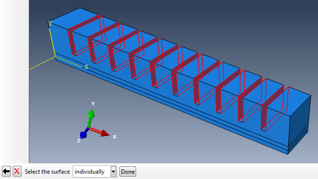
Now, we select the surfaces where the contact will occur. Select all the adjacent chamber walls in the actuator, by clicking on the relevant faces while holding down SHIFT on your keyboard. You will need to rotate your view at least once to select everything. Click the 'Done' button when finished.
One last "Edit Interaction" window will pop up. Use the default settings, seen below:
Mesh
Create mesh
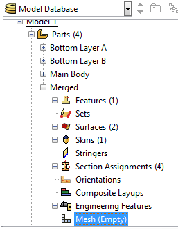 |
Expand the Merged part in the model tree and double-click on Mesh. |
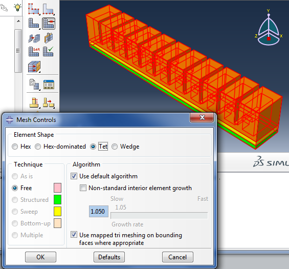
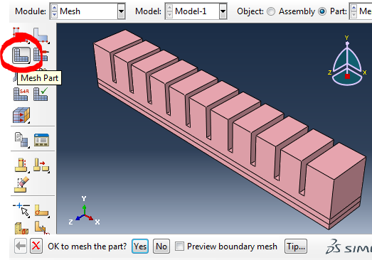
Click the ‘Mesh Controls’ button in the toolbar, then select all the parts of the assembly. In the window that pops up, select 'Tet' for the element shape.
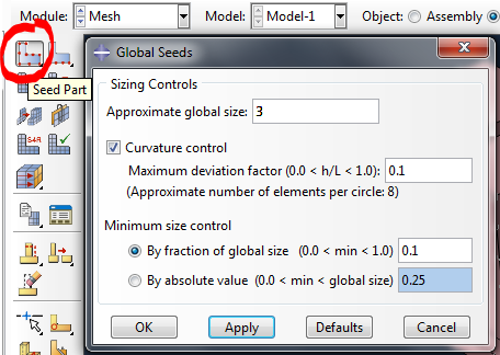 |
Seed the part with an ‘Approximate global size’ of your choosing. If the mesh size is too small, the model may become “stiff” to high distortions. But if it is too big, the mesh will not fit on well on the model face. Here we use a size of 3. |
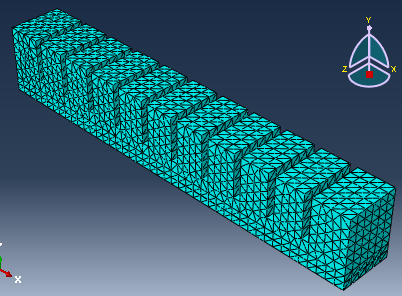
Mesh the part.
Set mesh type
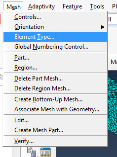 |
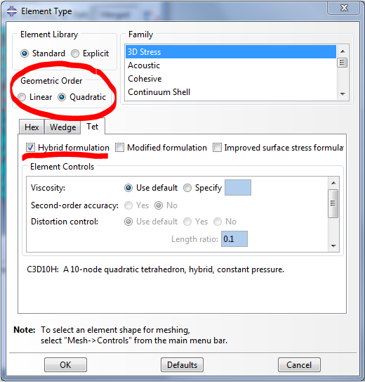
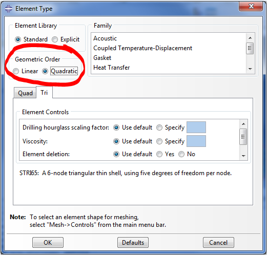
Because we are using a hyperelastic material, a Hybrid element type for the mesh should be used. In the menu bar at the top of the Abaqus window, go to Mesh → Element type, then select the 3 parts for the region (click one by one so you don't include the paper layer). |
Activate the tick on ‘Hybrid Formulation’ for all the hyperelastic parts. Make sure ‘Geometric Order’ is Quadratic.
Now do the same for the skin (inextensible layer). First, isolate the surface using the Display Group Manager as before, then again go to Mesh > Element Type. In the new window, change the Geometric Order to Quadratic so that it matches the other elements.
Run job and view results
Run job
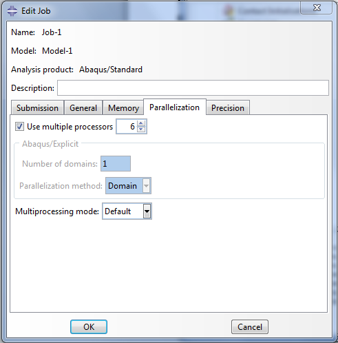 |
[Video: Create, submit and monitor job] Now, we are ready to submit the job and run the simulation. In the model tree, under Analysis, double-click on Jobs to create a new job. You can use the default settings, or change certain options (i.e. multiple processors) so that Abaqus can use more computer resources and complete the job faster. |
Right click on the newly created job and select Submit.
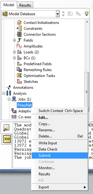
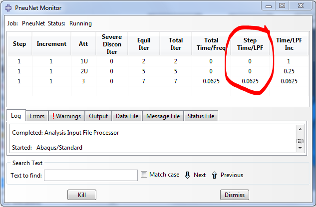
You can monitor the progress of the simulation by right clicking on the job and selecting Monitor. A new window will pop up. In the Step Time/LPF column you can see the percentage completion of that step.
View results
Once the simulation finishes, you can observe and analyze the results by right clicking on the job you just ran, and selecting Results. If you need to keep your results, they are saved in a large .odb file, typically in the TEMP folder or in the same directory as your model (.cae) file.
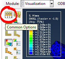 |
There are a several things you can do when viewing results. For example, clicking Common Options lets you tweak the appearance of the model result (i.e. shading, wireframe view, etc.) |
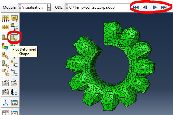
To see what the actuator looks like after gravity and pressure have been applied, click on Plot Deformed Shape. The navigation arrows in the top right corner of the screen allow you to scroll through the step increments and see how the actuator reaches its final shape.
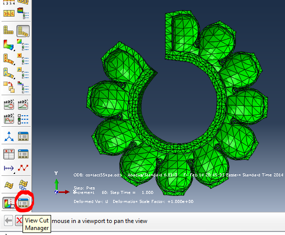
You can use the View Cut Manager to see section views of the deformed actuator, and use the button next to it to easily toggle the view cut on and off.
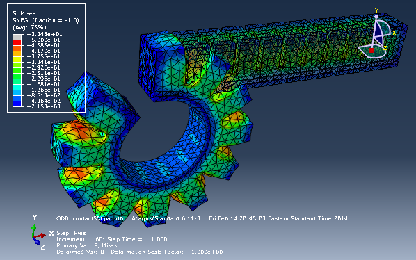
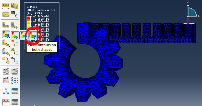
You can Plot Contours on both shapes (click and hold the toolbar button to make this option available), which superimposes the initial and final actuator shapes. This also lets you see the actuator color-coded by stress (Mises). Note that the actuator looks entirely blue (low end of the scale); this is because the highest stresses are in the paper layer, which is not visible, which affects the relative scale that Abaqus uses to color-code the model.
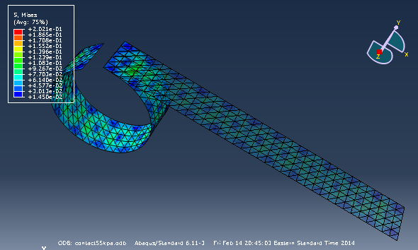
We can verify this by using the Display Group Manager again to isolate the paper layer, and now we can see the color-coded stress.
To see color-coded stress in different areas of the elastomer body of the actuator, we can manually change the scale using Contour Options. Note that by default, the scale limits are auto-computed by the minimum and maximum values in the model results.
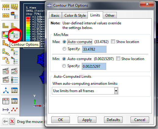
Try specifying the maximum value as 0.5 and note that now you can see the stress color-coding in the actuator.