Modeling
As mentioned in design section, wall thickness and groove depth in the design of the honeycomb structure can affect the mechanical performance of the manipulator. In this section, we propose two evaluation metrics for assessing the mechanical property of the manipulator, flexibility and load bearing capacity. After that, we use FEM modeling method to analyze this metric for segments with different thickness and groove depth, which can provide guidance for implementing a real manipulator.
For the whole manipulator, the flexibility is imperative for its front portion of the manipulator while the load bearing capacity is imperative at its base. By comparing the performance of different structures in simulations, we are able to understand the relationship between the performance (flexibility and load bearing capacity) of the manipulator and design parameters (wall thickness and groove depth).
|
|
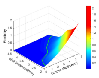
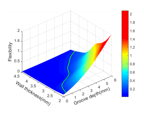
The variation of flexibility is illustrated in the figure above (left). We find that as the groove depth grows, the flexibility increases, while as the wall thickness grows, the flexibility decreases. Both variations are monotonous.
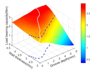
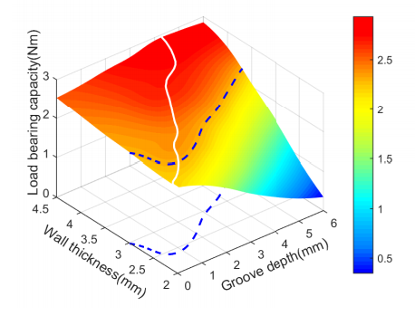
As shown in the figure on the right, the load bearing capacity increases monotonously as the wall thickness grows. However, the variation of load bearing capacity about the groove depth is not monotonous: it initially increases, and then decreases.
All of this will be detailed in evaluation, FEM simulation process and resulting analysis of the parts.
Evaluation
There are kinds of soft manipulators that achieve appreciable performance in their specialty respectively, nevertheless, there isn’t a universal evaluation criteria for assessing and comparing their performance. In this page, aimed at reaching a high level of load bearing capacity with little loss in flexibility, we set these two characteristics as the main metrics.
Flexibility
As for flexibility, we define it as a manipulator’s reachable space, which consists of all the points that the tip of the manipulator can reach with another end fixed. To show comparison between manipulators with different shapes and scales, we calculate the ratio of that space to the dimensionality’s power of its original length, as a relative flexibility.
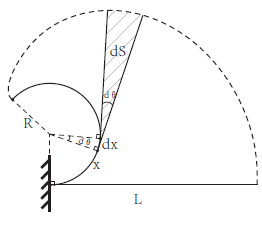
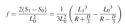
Minimum bending radius, original length, maximum length and width of the manipulator are represented as R, L0, L1 and D respectively. S1 is the bending arc and outer boundary and S0 is the bending arc and inner boundary.
Load bearing capacity
As for load bearing capacity, we define it as the maximum load moment of a soft manipulator when it is able to remain stable and its loaded end is on the same height with its fixed end. How the manipulator reaches such a condition is not confined.
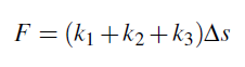
F represents the internal force provided by the airbags, which is determined by the contact area S and pressure p. k1, k2, k3 represent the spring coefficients, M represents the load moment provided by this structure. To reach a balance, we assume a elongation of Δs for the springs.
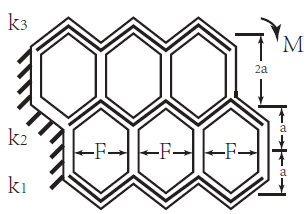
The force balance can be represented as:
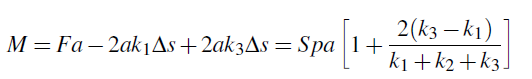
The load moment can be calculated as:
Finite Element Modeling (FEM)
This section describes how to perform Finite Element Method (FEM) analysis of our PneuNet actuator using the Abaqus software suite.
Overview of model components
-
2 materials:(because wo notice at structure,so material can be imprecise)
- frame: polyflex density of 1200Kg/m³,a Young’s Modulus of 0.1 GPa and a Poisson’s ratio of 0.38
- airbag: PA+PE density of 1200Kg/m³,a Young’s Modulus of 1 GPa and a Poisson’s ratio of 0.45
-
2 sections:
- frame(uniform solid), assigned to the frame
- airbag (uniform shell), assigned to airbag
Overview of FEM steps
- Import parts
- Assign material properties to the parts (create materials, assign materials to sections, assign sections to parts)
- Assemble parts
- Create step
- Create a universal contact
- Create set and surface
- Apply loads and set boundary conditions
- Mesh part
- Create mesh and run job
Abaqus units
When the lang unit is 'mm' ,the other unit is detemined

FEM for Load Capacity
In this section, we are mainly concerned with the impact of groove depth and wall thickness on the load.
3 loads:
- Step-1: pressure and concentrated force
- Step-2: a contrary concentrated force
So, we can finally get the side of the airbag when fully Inflated, the arm can maintain the level of the load.
Then wo can get the load moment which represents the load capacity of this structure.
Cae here
Import Parts
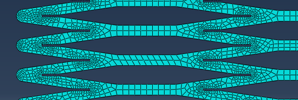
In this project, as mentioned in the Design section, we only consider the characteristics of the manipulator in x-y plane. And thanks to the structural property, we only analyze a slice of the frame (as shown below) instead of the whole structure, which can make the simulation much less computationally expensive.
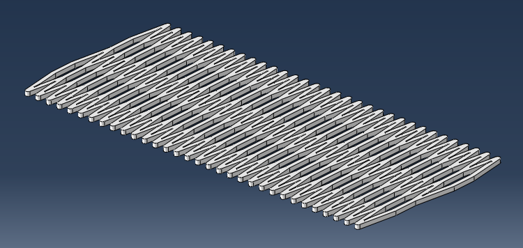
The .stp files of the simplified geometry used in this tutorial can be downloaded here.
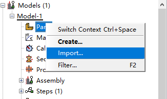
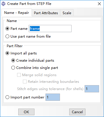
Import frame
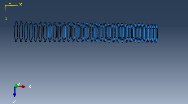
To import the fram go to the model tree in the left sidebar, right-click on Parts and select Import. Browse to the frame.stp file. The frame here has a little difference from the CAD tutorial model: the chambers' number is 64 instead of 16, and the extruded height is 2 mm instead of 60 mm.
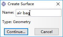
Create airbag
Create a new part named 'air bag' and select Shell and Extrusion.
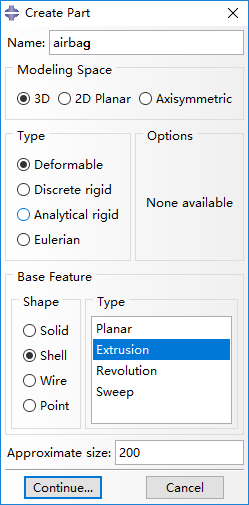
The slice of a airbag should be with an ellipse shape, but we design the airbag as illustrated below for convenience of adding interactions (mentioned later).
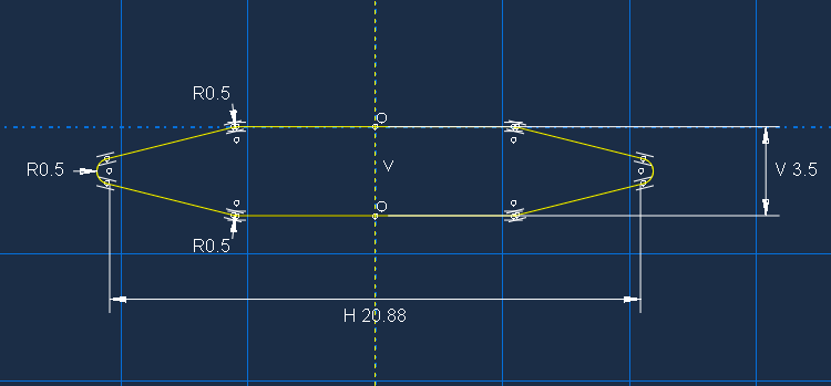
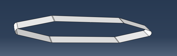
Set the Depth of this extrusion as 20 and the part of airbag is shown below.
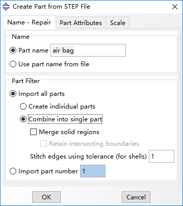
You can also directly import the part from .stp file and select Combine into single part.
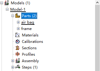
Finally, two parts should now appear in the model tree.
Assign Properties
In this page, we will show detailed procedures of assigning material properties for frame and airbags.
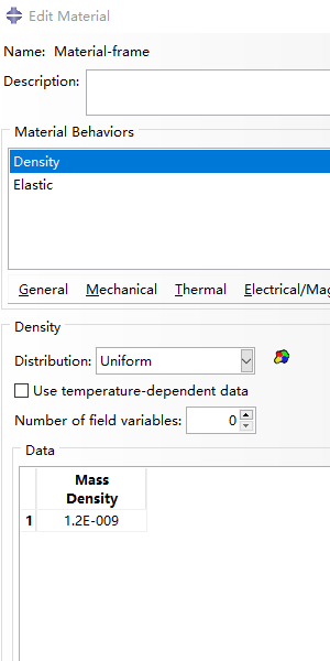
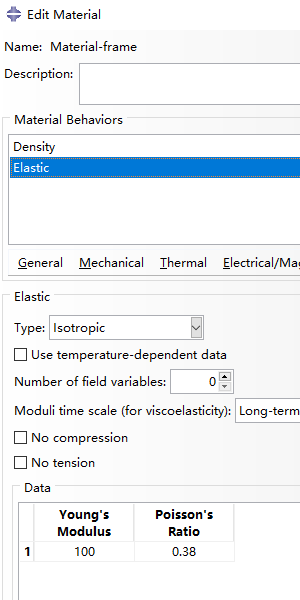
Create Material: frame
Firstly, we create a new material named 'Material-frame' for the frame. And set the following properties:
-
General > Density:
- Density = 1.2e-9 Mg/mm³
-
Mechanical > Elasticity> Elastic:
- Young’s Modulus = 100 MPa
- Poisson’s ratio = 0.38
|
|
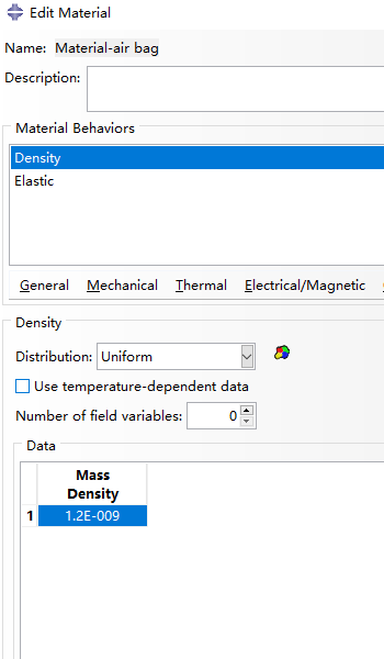
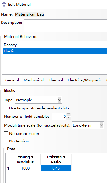
Create Material: airbag
For the property of airbags inside named ' Material-air bag', set:
-
General > Density:
- Density = 1.2e-9 Mg/mm³
-
Mechanical > Elasticity> Elastic:
- Young’s Modulus = 1000 MPa
- Poisson’s ratio = 0.45
|
|
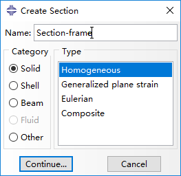
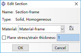
Create Sections
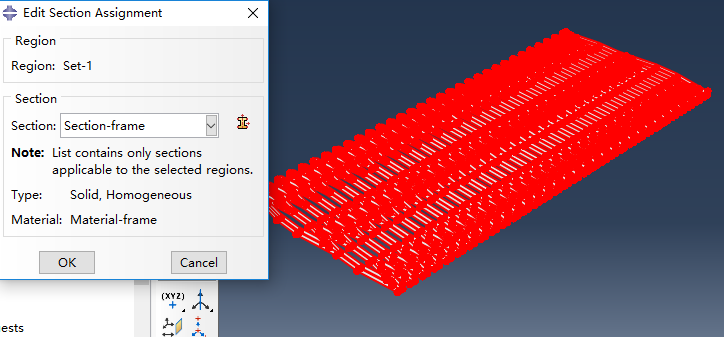
Double click on Sections in the model tree to create a new section. Set it to be a homogeneous solid and assign 'Material-frame' as its material.
|
|
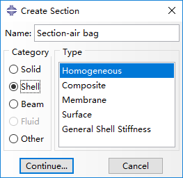
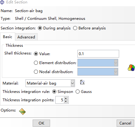
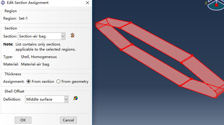
Create another section and set it to be a homogeneous shell and assign 'Material-air bag' as the material. Set the shell thickness as 0.1.
|
|
Edit Section Assignment
Last, assign the section property to corresponding part by selecting the entire part geometry.
Assemble
In this page, we first create instances from the imported parts for 'frame' and 'air bag', move the air bag towards proper position, and then replicate airbags in each chamber of the manipulator frame.
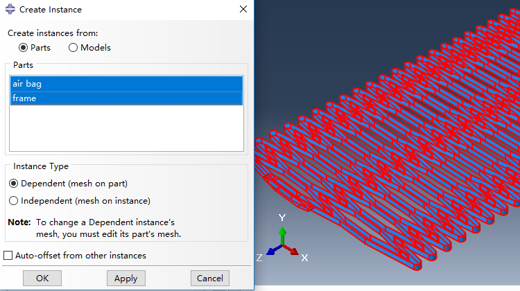
Create instance
Instances are created from imported Parts named 'frame' and 'air bag' in page 'Part', and we select instance type as Dependent (mesh on part).
Position air bag
Now the airbag has to be positioned properly. Firstly, the air bag is rotated 90 degrees around x-axis, forming a result posture shown as below.
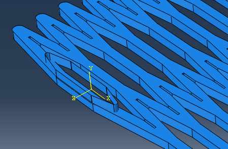
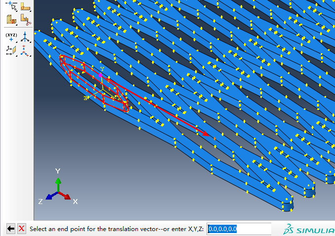
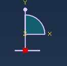
Next, the air bag should be translated into a chamber of the manipulator frame, which is implemented based on a translation vector from the magenta point towards the orange point illustrated below.
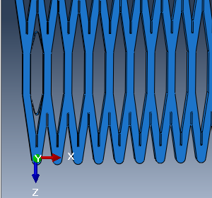
Then, we rotate the whole structure 90 degrees around y-axis, and the result is shown like this.
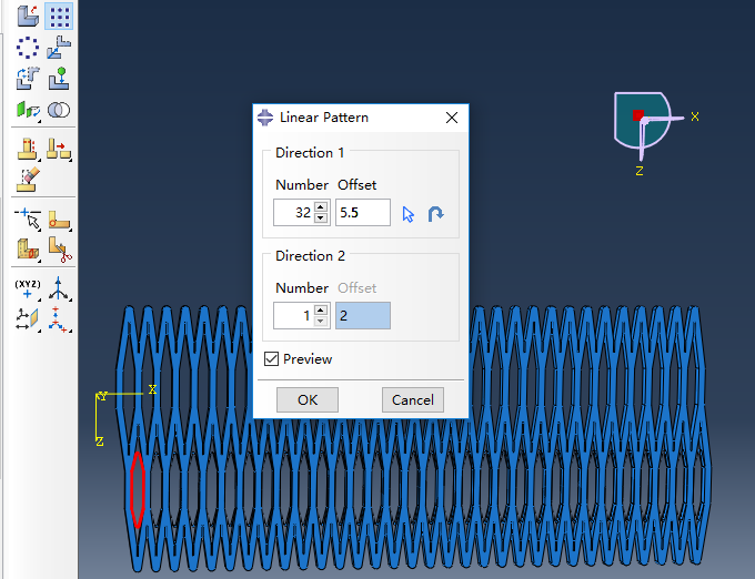
Linear pattern
Last, airbags are generated using Linear pattern, and set the Number as 32, Offset as 5.5 in Direction 1.
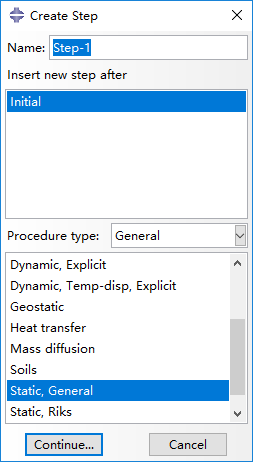
Create Steps
In this page, we create two steps, 'Step-1' and 'Step-2' for load simulations. 'Step-1' is created with procedure type of Static, General.
In the next window, turn on Nlgeom option in Basic panel.
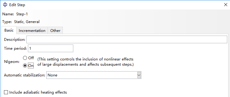
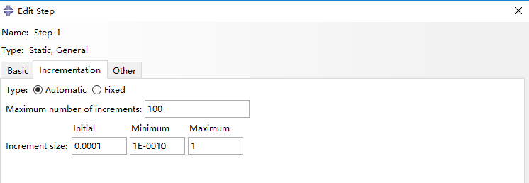
In Incrementation panel, we select type as Automatic, set Maximum number of increments as 100, and set Increment size as 0.0001, 1e-10 and 1 respectively for Initial, Minimum and Maximum.
|
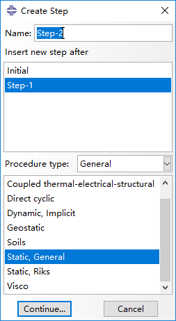
Next, 'Step-2' is created after 'Step-1', also with procedure type of Static, General.
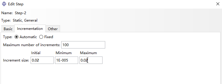
'Step-2' also needs enabled Nigeom in Basic panel. In Incrementation panel, we select type as Automatic, set Maximum number of increments as 100, and set Increment size as 0.02, 1e-5 and 0.02 respectively for Initial, Minimum and Maximum. Notice that the Maximum increment size of 0.02 here is set for convenience of the result analysis afterwards.
Add Contact Interaction
Create interaction property
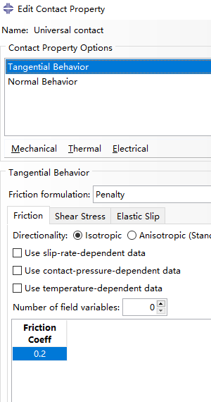
First, we create the type of interaction we want to model. In the model tree, double click on Interaction Properties and create a new property of the type Contact, named 'Universal contact'.

Add Mechanical > Tangential Behavior from the dropdown menu, and set friction coefficient as 0.2 (this parameter is of little importance).
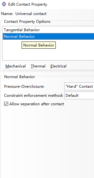
Next, add Mechanical >Normal Behavior as shown below.
Create interaction
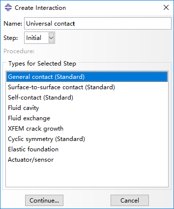
Then create an interaction named 'Universal contact', beginning from step 'Initial' with type of General contact (Standard).
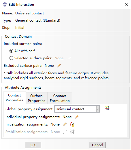
Last, edit interaction by selecting All* with self for included surface pairs, Universal contact for global property assignment in Contact Properties panel.
Create Loads
Create sets and surfaces
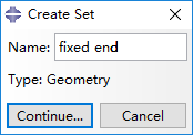
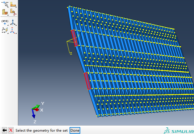
Firstly, we create a new set named 'fixed-end', by clicking 'Tools > Set > Create' button.
Continue and click on the faces (red) of the part that is going to be fixed.
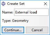
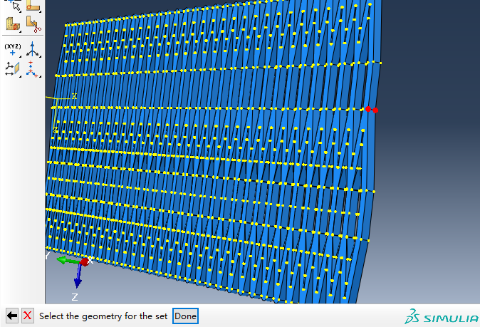
Repeat the operations above to create a new set called 'External load'.
Continue and select the two points (red) to be exerted force.
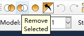
Then, we hide the frame using the button Remove Selected, only appearing airbags as the figure below.
Next, we create another set named 'air bag' by clicking 'Tools > Set > Create' button again.
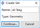
Continue and select all the airbags as a set that is going to be constrained afterwards.
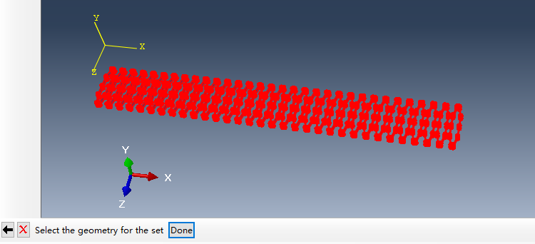
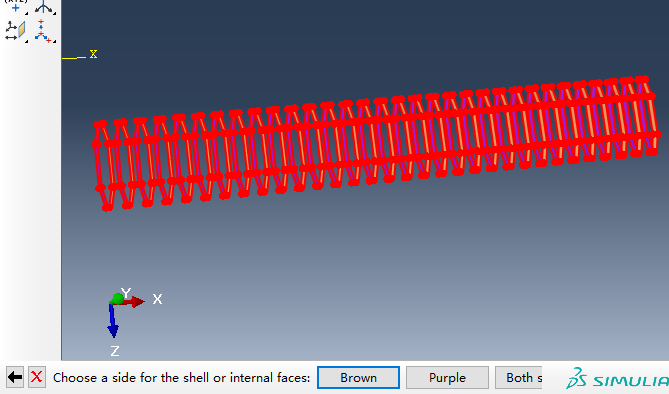
Then, create a surface also named 'air bag' by clicking 'Tools > Surface > Create' button.
Click 'Brown' to select the internal face of these airbags.
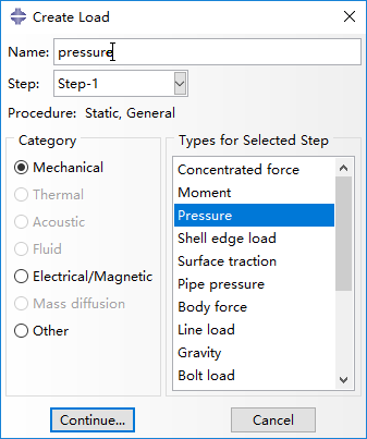
Create loads
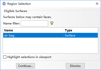
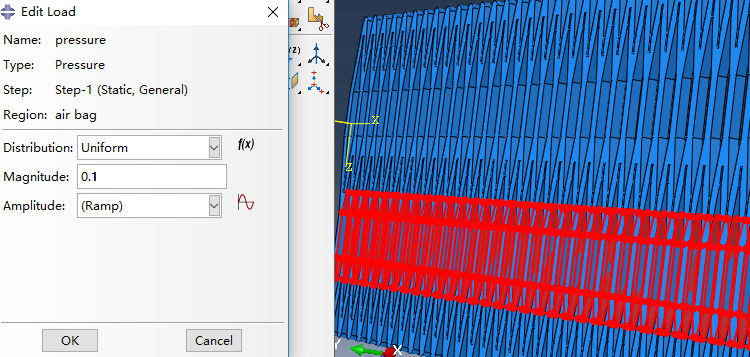
Under the 'Step-1', create a load named 'pressure' and activate Pressure as the selected type for the step.
In the Region Selection window that appears, select the surface 'air bag' which we created earlier.
At the next window provide the pressure value to be applied in the airbags by setting Magnitude as 0.1 Mpa.
Next, we create a load of external force in 'Step-1' named 'External load' with type of Concentrated force.
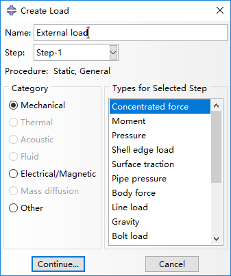
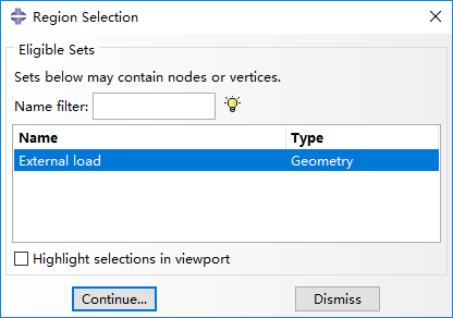
Select set 'External load' which we create earlier.
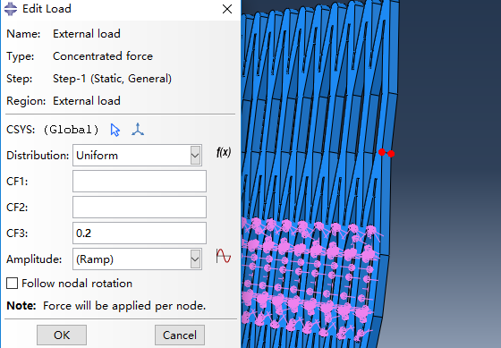
Continue and set CF3 as 0.2 N exerted on the two points (red) at the manipulator's tip.
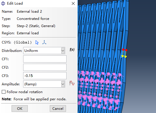
Then, create another external load named 'External load 2' in 'Step-2' with types of Concentrated force.
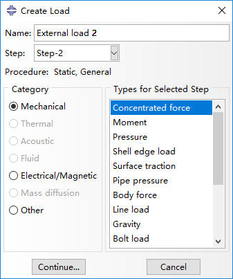
This load is implemented as a force in the opposite direction of the prior one, with a magnitude of 0.15 N (CF3 set as -0.15).
Set boundary conditions
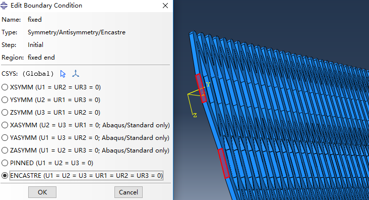
Create a new boundary condition named 'fixed' in step 'initial' and select Symmetry/Antisymmetry/Encastre.

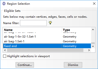
In the next window select set 'fixed end'.
And select ENCASTRE to fix the red regions.
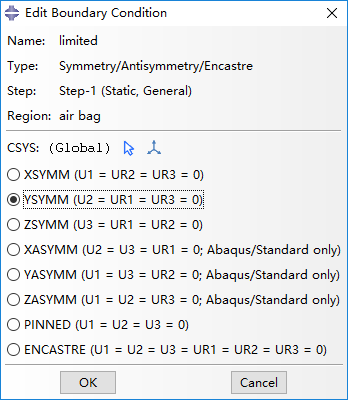
Next, create new boundary condition named 'limited' in 'Initial', with the same property as the prior.
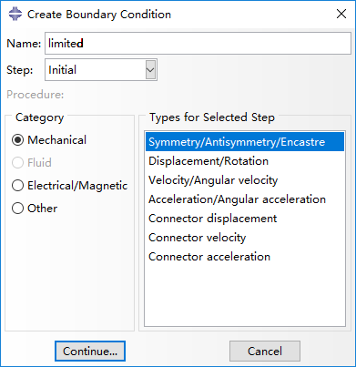
And select YSYMM to make airbags unable to move in y-axis.
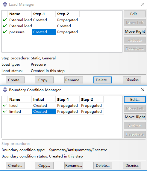
Finally, we can check the load, boundary information in Load Manager and Boundary Condition Manager.
Mesh
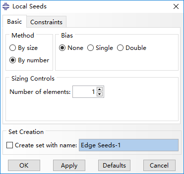
Seed edges
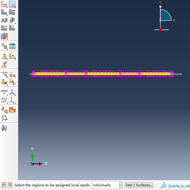
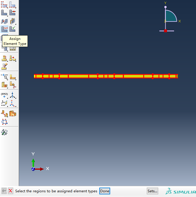
Firstly, select Part in upper right panel and choose 'frame'. Click Seed Edges (button with shaded background in the figure) and select all the edges.
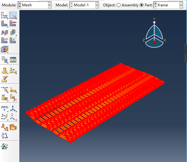
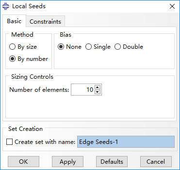
In the new window, we set the Number of elements as 10, which means each edge has 10 seeds.
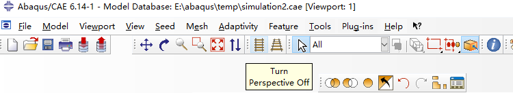
Then, convert the perspective by clicking at z-axis.
And click Turn Perspective Off.
Because the slice is thin enough, we change the seeds on these edges along y-axis to 1.
Mesh
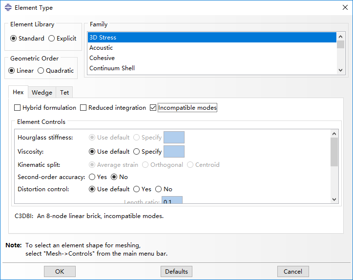
Next step, click Assign Element Type button.
Enable Incompatible modes option, with other options set as default. Thus, the mesh type is C3D8I, as shown below.
Then click Mesh Part Instance and get the meshed frame as shown below.
The mesh of airbag can be implemented in a similar way. The result is illustrated like this.
Run Job and Result Processing
Run job
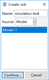
Firstly, we create a new job named 'simulation-test'.
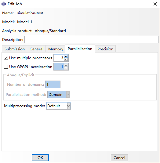
You can use the default settings, or change certain options (i.e. multiple processors) so that Abaqus can use more computation resources and complete the job faster.
Then Submit the job.
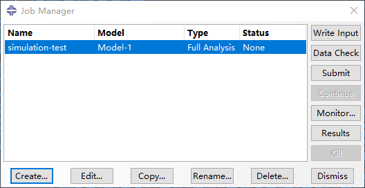
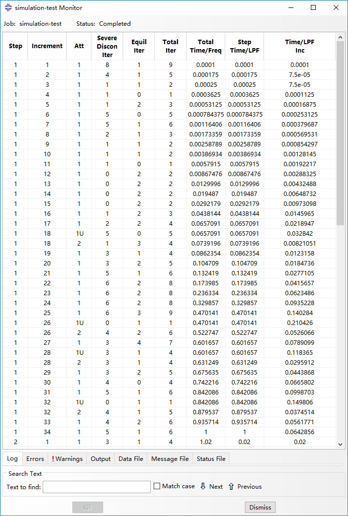
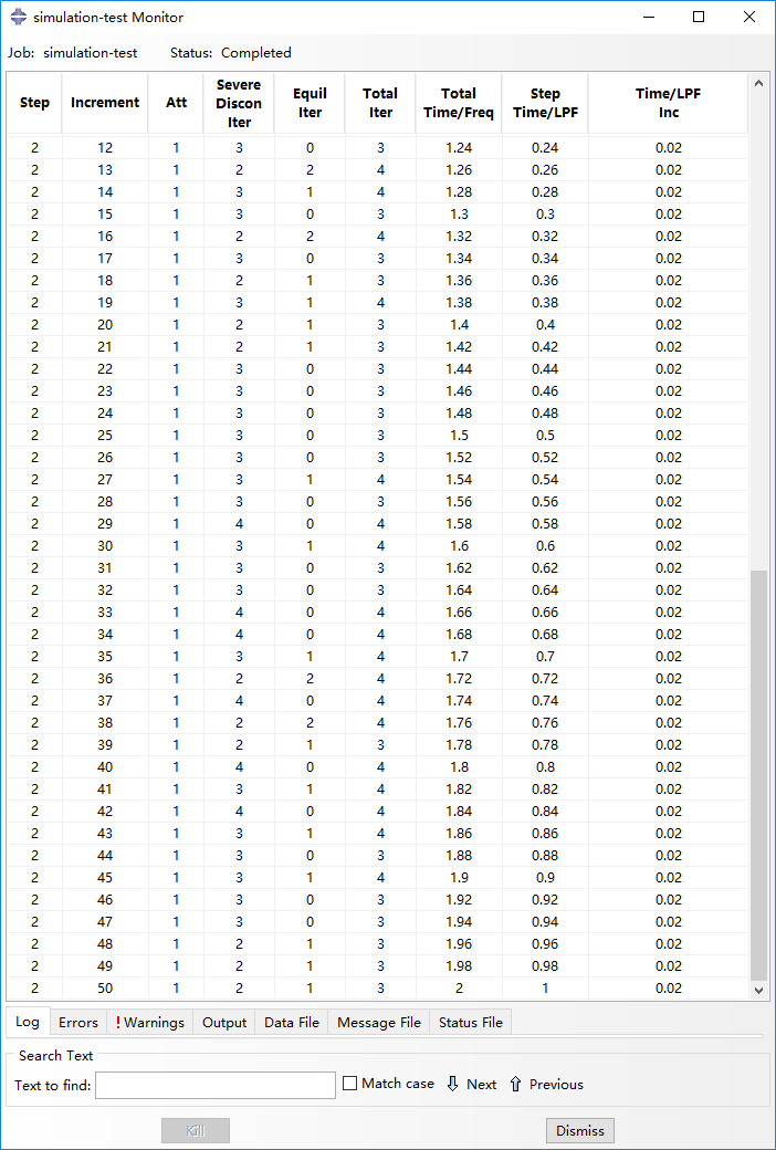
You can monitor the progress of the simulation by clicking on Monitor. A new window will pop up. In the Step Time/LPF column you can see the completed percentage of that step.
Result processing
Once the simulation finishes, you can observe and analyze the results by clicking on the Results. If you need to keep your results, they are saved in a large .odb file, typically in the TEMP folder or in the same directory as your model (.cae) file.
In Visualization module, the navigation arrows in the top right corner of the screen allow you to scroll through the step increments and see how the manipulator deforms. The figure below shows that the manipulator finish Step-1, and at the beginning of Step-2.
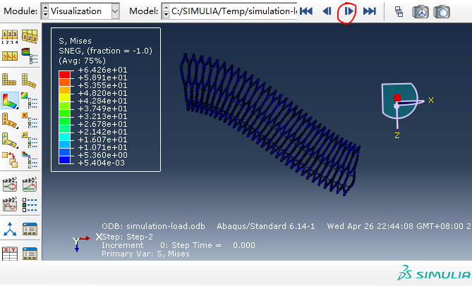
In homepage, we define the load capacity as the load moment when the manipulator's loaded end is on the same height with its fixed end, so we continue to click navigation arrows and use 'Tools > Query' to check the tip point's (red) displacement. As marked in red box, the tip point's displacement in the z-axis is -1.85mm when the time equals 0.52, which can be approximated that the tip has reached the same height with fixed end.
Thus, the load on the manipulator's tip can be calculated as (0.2 - 0.15*0.52)*2 = 0.244 N. Notice that the load is gradually exerted and proportional to step time. Besides, the force is exerted on two points, so it's multiplied by 2.

Then, use Distance to get the distance (248mm) between two selected points.
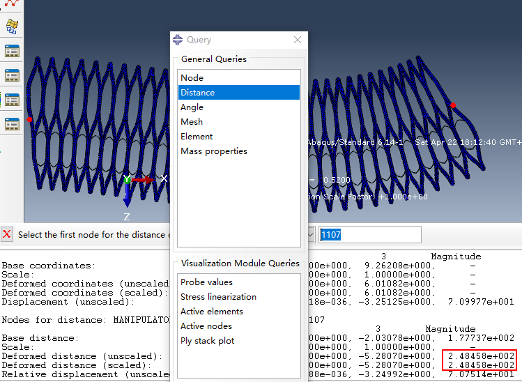
So, the moment is calculate as 0.244*0.248 = 0.0605 N/m. This value is calculated under a 2 mm thickness condition. For the real structure, the thickness is 60 mm, so the real moment is about 0.0605*60/2 = 1.82 N/m.
FEM for flexibility
In this section, we are mainly concerned with the impact of groove depth and wall thickness on the flexibility.
Cae here
Because all the operations have been introduced in the previous section, we will only show the difference.
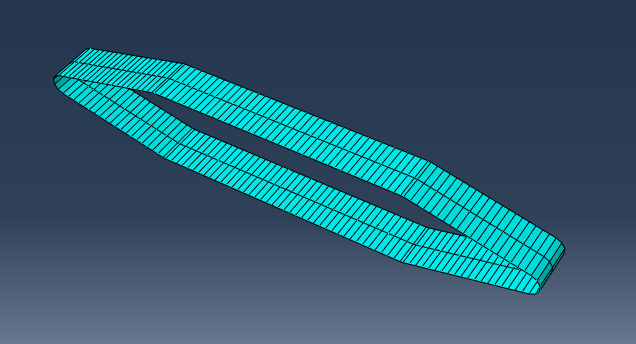
The following is our Assembly.
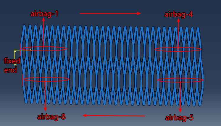
9 loads:
- Step-0: all airbag 0.001Mpa(The airbag establishes contact with the arm)
- Step-1: airbag-1 0.1Mpa
- Step-2: airbag-2 0.1Mpa
- Step-3: airbag-3 0.1Mpa
- Step-4: airbag-4 0.1Mpa
- Step-5: airbag-5 0.1Mpa
- Step-6: airbag-6 0.1Mpa
- Step-7: airbag-7 0.1Mpa
- Step-8: airbag-8 0.1Mpa
So, we can get the result like this.
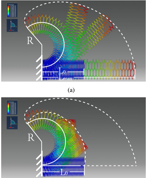
We measured that area using Monte Carlo method. Furthermore, using L0, L1, R and D, the reachable space can be calculated by the formula. The calculated area approximately equals to the measured counterpart, which validates the calculation method.
(Advanced) Result Analysis
|
|
The variation of flexibility is illustrated in the figure above. We can find that as the groove depth grows, the flexibility increases, while as the wall thickness grows, the flexibility decreases. Both variations are monotonous.
As shown in the figure, the load bearing capacity increases monotonously as the wall thickness grows. However, the variation of load bearing capacity about the groove depth is not monotonous: it initially increases, and then decreases. We believe the cause is that as the groove depth increases, then the arm of gravity and load increases while the forces themselves decrease. Because the wall of a relatively large thickness confines the airbags’ inflation, the forces decrease slowly when the groove depth is relatively small. So their product initially increases.
Besides, the deformation of airbags is confined, so the increasing forces' of the arm is confined while the forces always decrease as the groove depth increases. So their product has an extreme value, and then decreases. Because of the non-monotonous variation, the load bearing capacity reaches an extreme value at a certain groove depth under every fixed wall thickness (white line in the right figure). On its left side, the flexibility and load bearing capacity both increase as the groove depth grows. Thus, values in this region are not concerning because both properties can be better on the right side of the white line.
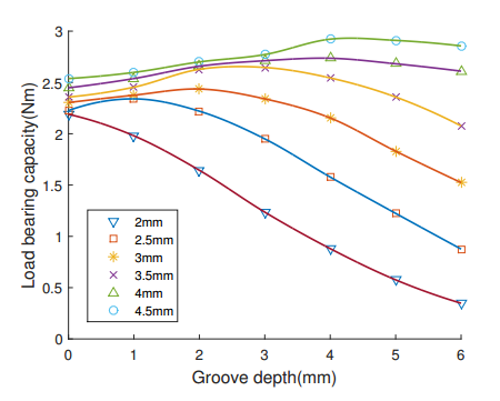
To get an explicit view of the load bearing capacity’s non-monotonous variation along with the groove depth, the performance of load bearing capacity under different fixed wall thickness are demonstrated in 2D plane in the figure below. From that, several conclusions can be drawn:
• As the wall thickness grows, the extreme point moves rightwards, so a deeper groove is required corresponding to a thicker wall for achieving maximum load bearing capacity.
• The curve corresponding to a 2mm wall thickness monotonously declines, with no extreme point. From the trend that the extreme point moves leftwards when wall thickness decreases, we can infer that when the wall thickness is less than a certain value, the extreme point has a minus groove depth. Therefore, an additional part at the intersection, instead of a groove, is required to realize a model with a thin wall.
• With a fixed groove depth, the load bearing capacity always increases as the wall thickness grows, but its rising range gradually reduces. So, it’s not effective to keep increasing the wall thickness when it’s already large. Instead, it is useful to increase the pressure.