Testing
To test and calibrate the sensor we used objects with known lengths to press against the sensor placed on top of a load cell.
Overview
As seen in the video, the sensor was loaded with wooden sticks of various lengths. Force was manually applied until the electrical resistance of the sensor changed. To monitor this changes in real-time we used the Robot Operating System (ROS) as a backend for our data collection. Using ROS eases systems integration across multiple systems and hardware. We will not go into detail on how the systems integration is performed.
Disclaimer: The raw data feed shown in the video was collected in a seperate but similarly performed data collection session.
Testing hardware
- National Instruments USB-6351 Data Acquisition (DAQ) system for measuring resistance
- Teensy 3.5 for reading pressure sensor
- LoadStar iLoad Pro
- Various sections of wooden sticks with known length
Testing software
- Robot Operating System
- rosserial_python
- LabVIEW & LabVIEW ROS
Raw Sensor Data
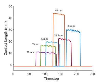
The raw data from the sensor is in two separate data streams: the resistance (the voltage drop) and the pressure. Plotted below are raw (zeroed) readings from the sensor - similar to what is shown in the overview video.
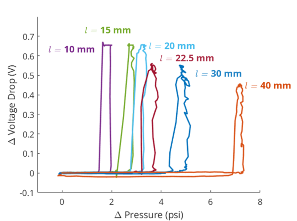
The sensor was loaded as shown in the above video. We recorded a continuous datastream for all measurements and sectioned the data time-wise according to the object impinging the sensor.
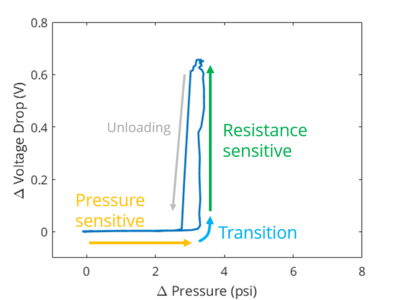
The sensor exhibits an interesting behavior where the voltage drop (resistance) starts changing as the pressure increase starts to saturate. The point of transition from pressure to voltage drop sensitivity depends on the contact area of the object impinging the sensor. Using this knowledge, and the ground truth data (the loadcell), we can calibrate the sensor in the following modalities.
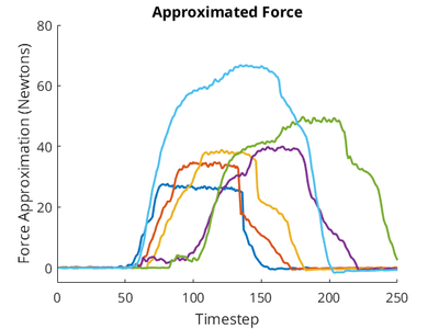
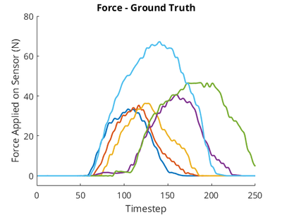
Force
As the voltage drop (or resistance) picks up in sensitivity after the pressure change saturates, we use the following formula for derving the force applied to sensor:
\(F=(P+V\times K_C)\times K_F\)
where:
\(F :\) force
\(P:\) pressure
\(V:\) voltage drop
\(K_C:\) calibration constant
\(K_F:\) calibration constant
\(K_F\) is approximate from the following linear fit, where the raw value is \(F=P+V\times K_C\) where \(K_C\) is 0.21 (heuristically found). We used a \(K_F\) of 8.16.

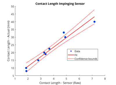
Contact Area
As we used objects that are larger than the width of the sensor, we can use the length of the object in contact with the sensor instead of the area. Since the voltae drop starts to change at a particular pressure for each object length, the formula for deriving the contact length is:
\(l = P \times (V > V_{threshold}) \times K_A\)
where:
\(l :\) contact length
\(P:\) pressure
\(V:\) voltage drop
\(V_{threshold}:\) threshold voltage
\(K_A:\) calibration constant
For the sensor in the guide, we used \(V_{threshold}=0.3\) and \(K_A =6.22\). For clarification \((V>V_{threshold})\) is 1 if V is greater than the threshold voltage and 0 if not.
From our recorded data, we can plot the following. It is clear that the sensor can discern between objects of various sizes given the object applies enough force to the sensor to trigger the transition.
Our \(K_m\) is derived from the following linear fit
Bibliography
Preechayasomboon et. al. Multi-Modal Sensing and Actuation in Biomechanical Hydraulic and Pneumatic Systems.
Contributors
Pornthep Preechayasomboon
Gaurav Mukherjee
Eric Rombokas