Finite Element Analysis Modeling
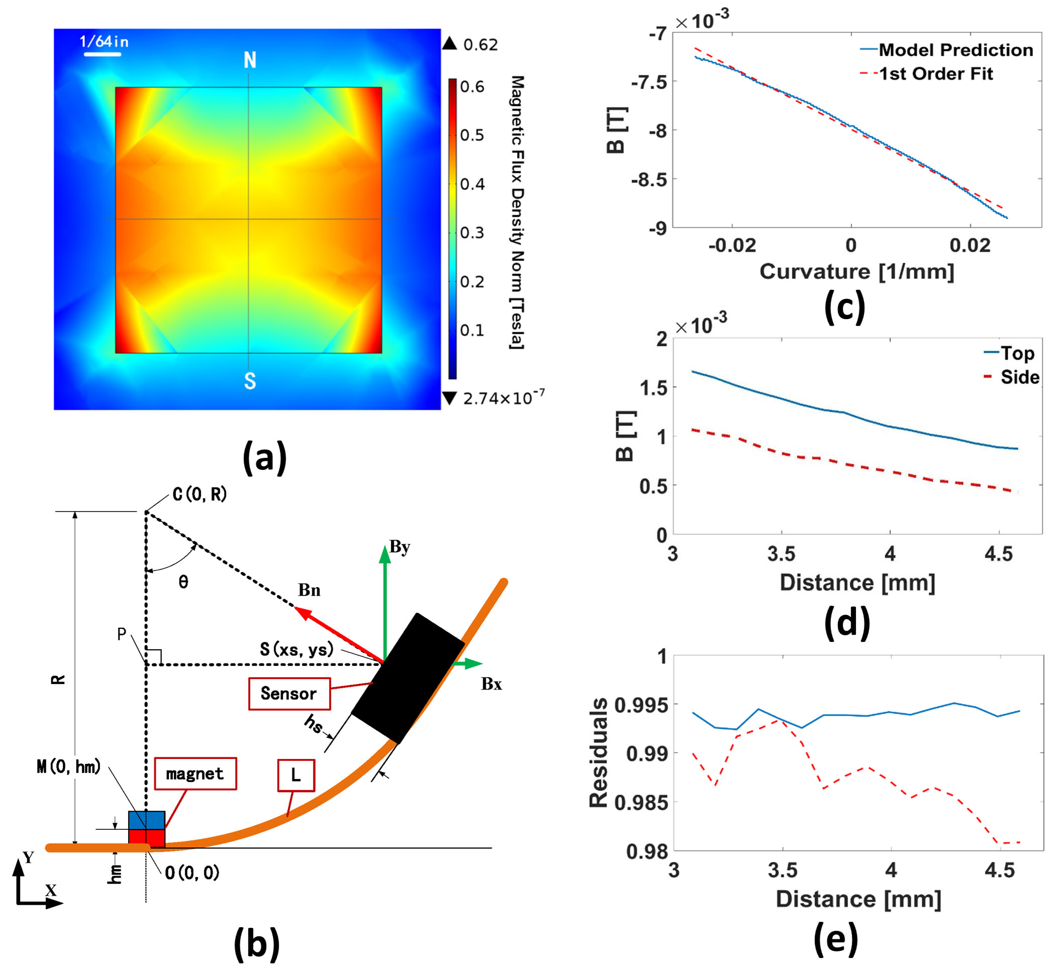
This section shows how to choose the optimal design for curvature sensor. We considered two main parameters: the orientation of the magnet and the distance between the magnet and the Hall element. First, we generated magnetic field data using COMSOL, an example of which can be seen in Figure 13a. We used this to calculate the strength of the magnetic field at the Hall element with respect to the circuit design. Figure 13b shows the geometric relationship between the magnet and the Hall element on a bending segment. The origin is located at the base of the magnet, L is the arc-length along the flexible circuit between the origin and the center of the Hall element, hm is the height of the center of the magnet (point M), and hs is the height of the Hall effect sensor element (point S). We assume that the flexible sensor is under constant curvature, allowing us to calculate the positions of these two points.
We can calculate the vector between M and S, and then use the COMSOL magnetic field data Bx and By at S to determine the expected field registered by the Hall element (in its normal direction) via the following rotation equation:
Bn=BycosΘ-BxsinΘ
where Bn is the magnetic field density, which the onedimensional Hall effect sensor could sense when the bending angle is h. When analyzing the sensor simulation, we considered the working range of the bending actuator to be 90, representing the bounds of h. Figure 13c shows the model prediction of the magnetic field with respect to curvature at a distance of L ¼ 3.1 mm, the results of which can be approximated using a linear fit. To determine the optimal distance and magnet orientation, we calculated the range of measured magnetic fields for L ranging between 3.1 and 4.6 mm with the magnetic north pointing upward (along y-axis) and sideways (along x-axis), the results of which can be seen in Figure 4d.This range was chosen to keep the sensor from coming into contact with the magnet at larger curvature values, as well as keep the magnetic field from becoming too weak to be measured effectively. These sensor readings can each be approximated by a linear fit, as in Figure 13c. We compared the residuals (R2 values) for these fits for top- and side-facing magnets for the same range of L, representing the linearity of the resulting data. The results of this analysis can be seen in Figure 13e. We conclude that the top-facing magnet orientation is superior, because the working range is 30% larger and the data are more linear. In addition, it is found to be advantageous to minimize L to maximize the range of magnetic field readings.